1. Rockets and missiles as orbiting projectiles
The rocket (or self-propelled missile) equations of motion differ from the projectile equations of motion in several important ways. First, for long-range missiles the curvature of the earth, and the change of gravity with altitude now matters, so we need to consider both in defining our vector equations. Thus the "-mg" gravity interaction must instead use Newton's law of gravity:$$ \vec{F}(\vec{r}) ~=~ -\frac{GMm}{\left | \vec{r}\right|^3} ~ \vec{r} $$
where \(
\vec{F},~\vec{r}\) are 3-vectors here:
\(\vec{r}= (x,y,z)\) relative
to the center of a spherical planet of mass M (earth in
our case), G=
6.67e-11 is the gravitational constant, and m is the
rocket mass.
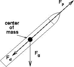
The rocket force law must also account for the propulsion force F p or "thrust" p of the rocket. Typical rocket thrust values are given as equivalent weights at sea level, in units of kg. This means that a thrust of p kg can just "levitate" (or balance) a mass of m kg at sea level.
To get the true force associated with a given thrust, you mutiply by the local sea level value of g = 9.8066 m/s^2, thus Fp = g p gives the true force in Newtons for a quoted thrust p in kg.
As the rocket uses up the fuel that is initially carried and burned to produce the thrust during its initial ascent stage, the mass decreases, usually in a linear way:
$$ m(t) ~=~ m_0 - m_f \frac{t-t_0}{t_b}, ~ t<t_b $$
$$ m(t) ~=~ m_0 - m_f, ~ t\geq t_b $$
where m0 is the initial launch mass of the rocket, m f is the mass of the fuel, and tb is the "burn time" of the fuel. Thus at times beyond the end of tb , the mass remains constant.
The third force on a rocket is of course the air drag force, which is the same as the hydrodynamic drag force we encountered in the baseball case, involving again the apparent wind, the cross sectional area A of the rocket, a shape-dependent drag coefficient Cd, and rho, the density of the air, which depends on altitude again. The drag force (from Bernoulli's law) is thus:
$$ \vec{F}_b ~=~ -b\left |\vec{v}_{app}\right | \vec{v}_{app}, ~ b = C_d A \rho / 2 $$
Here is a data file taken from the NASA
NSIS-E-90
Atmosphere
Model:
which gives the number densities ( of ozone, N2 and O2), mass density, and temperature, every two kilometers. When you have a data file such as this one, that is slowly changing with altitude, often the best way to determine the density vs. altitude for any arbitrary altitude is to use this data as a lookup table in your program, and use linear interpolation to get the values for altitudes between the tabulated points.
Linear interpolation, if you are not familiar with it, is the procedure of using a simple line y = mx + b to connect two data points (x1,y1) and (x2,y2) in a table of values, and then to extract intermediate values for the y coordinate at an intermediate x coordinate (between x1 and x2) by using the equation for the line (that is, you need to find the slope m and the y-intercept b for each of the connecting lines in the data).
3. The rocket equation
$$\Delta p ~=~ m(t) \Delta v_{r} + v_e \Delta m$$
and taking a differential with respect to time we get
$$\frac{dp}{dt}~=~ m(t) \frac{dv_{r}}{dt} + v_e \frac{dm}{dt}$$
and since \(\frac{dm}{dt}\) is also constant during the burn phase, we can treat the second term on the right-hand side as a constant external force -- the rocket thrust -- during the burn phase. This allows us to recover Newton's force law using the remaining term, combined with other external forces such as the drag and gravity.
$$ \frac{d\vec{v}}{dt} ~=~ \frac{1}{m(t)} \left [ \vec{F}_g(\vec{r}(t)) + \vec{F}_b(\vec{v}(t)) + \vec{F}_p(m(t)) \right ] $$
The rocket force law must also account for the propulsion force F p or "thrust" p of the rocket. Typical rocket thrust values are given as equivalent weights at sea level, in units of kg. This means that a thrust of p kg can just "levitate" (or balance) a mass of m kg at sea level.
To get the true force associated with a given thrust, you mutiply by the local sea level value of g = 9.8066 m/s^2, thus Fp = g p gives the true force in Newtons for a quoted thrust p in kg.
As the rocket uses up the fuel that is initially carried and burned to produce the thrust during its initial ascent stage, the mass decreases, usually in a linear way:
$$ m(t) ~=~ m_0 - m_f \frac{t-t_0}{t_b}, ~ t<t_b $$
$$ m(t) ~=~ m_0 - m_f, ~ t\geq t_b $$
where m0 is the initial launch mass of the rocket, m f is the mass of the fuel, and tb is the "burn time" of the fuel. Thus at times beyond the end of tb , the mass remains constant.
The third force on a rocket is of course the air drag force, which is the same as the hydrodynamic drag force we encountered in the baseball case, involving again the apparent wind, the cross sectional area A of the rocket, a shape-dependent drag coefficient Cd, and rho, the density of the air, which depends on altitude again. The drag force (from Bernoulli's law) is thus:
$$ \vec{F}_b ~=~ -b\left |\vec{v}_{app}\right | \vec{v}_{app}, ~ b = C_d A \rho / 2 $$
where b
is Bernoulli's coefficient, Cd
is the drag coefficient (unit-less and
of order 1 or less), A is the
cross sectional area, and the density
\(\rho\) is a function of the magnitude
of the radius vector from the center of
the earth, since the missile may get to
quite high altitudes. It depends only on
the magnitude since we assume spherical
symmetry for the earth; if we wanted to
be rigorously realistic, even the
density would depend where we were on
the (slightly non-spherical)
earth. Note that the drag force
must be handled very carefully in your
equations, as it was for the Baseball
study -- in particular, you should
include the possibility of a non-zero
wind velocity, since higher altitude
winds are often quite strong.
2. Atmospheric Density function
The density function is also not as simple in the rocket case as it was for the baseball, since the atmosphere does not obey a simple exponential function over the wide range of altitudes required for a rocket. So we need a better model for the atmosphere. Here is a plot of actual atmospheric density vs. altitude:
which gives the number densities ( of ozone, N2 and O2), mass density, and temperature, every two kilometers. When you have a data file such as this one, that is slowly changing with altitude, often the best way to determine the density vs. altitude for any arbitrary altitude is to use this data as a lookup table in your program, and use linear interpolation to get the values for altitudes between the tabulated points.
Linear interpolation, if you are not familiar with it, is the procedure of using a simple line y = mx + b to connect two data points (x1,y1) and (x2,y2) in a table of values, and then to extract intermediate values for the y coordinate at an intermediate x coordinate (between x1 and x2) by using the equation for the line (that is, you need to find the slope m and the y-intercept b for each of the connecting lines in the data).
3. The rocket equation
3.1 A note on thrust
Before we can directly use Newton's force law for calculating rocket trajectories, we should be concise on what approximations we are using to make it applicable. We are assuming that rocket or missile thrust values are constant during the burn phase; this is a reasonable approximation but we have sidestepped the direct determination of thrust from the conservation laws. To do this, the change in momentum of the rocket must be equated to the change in momentum of the exhaust gas through the engine nozzles. Thus we locally conserve momentum in the following way. Suppose a small parcel of fuel \(\Delta m\) is exhausted at constant exhaust velocity \(v_e\) at time \( t\), resulting in a change in the rocket velocity of \( \Delta v_{r} \), then we have$$\Delta p ~=~ m(t) \Delta v_{r} + v_e \Delta m$$
and taking a differential with respect to time we get
$$\frac{dp}{dt}~=~ m(t) \frac{dv_{r}}{dt} + v_e \frac{dm}{dt}$$
and since \(\frac{dm}{dt}\) is also constant during the burn phase, we can treat the second term on the right-hand side as a constant external force -- the rocket thrust -- during the burn phase. This allows us to recover Newton's force law using the remaining term, combined with other external forces such as the drag and gravity.
3.2 Newton's law for rockets
The equation for the rocket acceleration is determined by summing these three forces and using Newton's 2nd law, thus$$ \frac{d\vec{v}}{dt} ~=~ \frac{1}{m(t)} \left [ \vec{F}_g(\vec{r}(t)) + \vec{F}_b(\vec{v}(t)) + \vec{F}_p(m(t)) \right ] $$
which provides the form
we need for the RK application, eg.:
dy/dt = f(t,y). Note here that there is
explicit dependence on r and v.
There is one important force missing from this equation, that is, at time t=0, the normal force is present to counteract the force of gravity, thus giving a boundary condition that you may need to be careful of depending on your implementation.
This is then a simplified form of the actual rocket equation, but complete enough for us to get realistic first-order trajectories. Some of the effects that it does not include are the lift forces, which are generated when the angle of attack of the rocket is not aligned with its velocity, and torque effects which arise when the forces act on moments of the rocket around its center of mass. There are many other details as well.
For those interested in precision rocket dynamics, take a look at Robert Stengel's Princeton website for Space System Design.
(Here is a PDF copy of the most relevant material)
For this assignment:
These plots should appear in your
final report (you will need to use
Xfig's "export" and make pdf or jpg or
png figure files).
Missiles have certainly been in the news lately for those of us in Hawaii, and of the greatest interest are the missiles of North Korea, which are detailed at this Federation of American Scientists site.
Use your equations and code to predict the maximum range of a 1-stage North Korean Nodong missile, which has the following parameters:
Determine the trajectory parameters that give you the maximum range.
What happens if the missile passes through the jet stream on the way up? Can you ignore its effects and still get an accurate answer?
Can you ignore the earth's curvature and still get accurate results here?
Extra Credit (25%)
There is one important force missing from this equation, that is, at time t=0, the normal force is present to counteract the force of gravity, thus giving a boundary condition that you may need to be careful of depending on your implementation.
This is then a simplified form of the actual rocket equation, but complete enough for us to get realistic first-order trajectories. Some of the effects that it does not include are the lift forces, which are generated when the angle of attack of the rocket is not aligned with its velocity, and torque effects which arise when the forces act on moments of the rocket around its center of mass. There are many other details as well.
For those interested in precision rocket dynamics, take a look at Robert Stengel's Princeton website for Space System Design.
(Here is a PDF copy of the most relevant material)
For this assignment:
- Modify your projectile (eg. baseball) code to create a new program called rocket.cpp or missile.cpp which implements the rocket equation with drag in vector form.
- Develop a linear interpolation function using the tabulated atmosphere above, to determine the density for any altitude of your rocket.
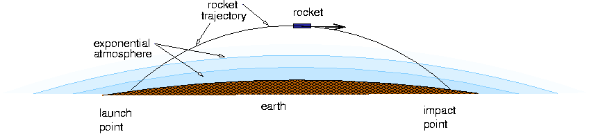
- Using Xfig, create a) a graph summary showing the vector forces on the missile, and b) a larger scale graph of the overall trajectory of the missile from start to finish, showing a curved earth, and something to indicate the decreasing density atmosphere. Your output should look something like this:
Missiles have certainly been in the news lately for those of us in Hawaii, and of the greatest interest are the missiles of North Korea, which are detailed at this Federation of American Scientists site.
Use your equations and code to predict the maximum range of a 1-stage North Korean Nodong missile, which has the following parameters:
- Thrust p = 26,051 kg
- launch mass m0 = 15,592 kg
- initial fuel mass mf = 13,326 kg
- burn time tb = 115 seconds
- diameter = 1.32 m (which determines the cross sectional area)
- drag coefficient Cd = 0.25
Determine the trajectory parameters that give you the maximum range.
What happens if the missile passes through the jet stream on the way up? Can you ignore its effects and still get an accurate answer?
Can you ignore the earth's curvature and still get accurate results here?
Extra Credit (25%)
Now that you have a functioning 1-stage missile simulator, try to modify this to do a two stage missile. This will require two burn periods since each stage carries a separate fuel load and has its own burn time.
Once you have this working, you are prepared to simulate a missile that is a real concern for those of us in Hawaii (and the US as well): the Hwasong-15: (these are approximate)
- Launch Mass: 70,500 kg
- 1st stage thrust (SI units): ~800 kN (average thrust including vacuum propagation)
- 1st stage fuel mass: 56,350 kg
- 1st stage burn time: 189 seconds
- 2nd stage thrust (SI units): 62.5 kN
- 2nd stage fuel mass: 5500 kg
- 2nd stage burn time: 220 seconds
- diameter: 2.40 meters
- drag coefficient: 0.25
- According to the source above, the maximum velocity as about 6700 m/sec, so you can use that to check your results.
- Does this missile have the range to hit Hawaii?
- Suppose it was required to hit a target area within a radius of 20 km, with no corrections in trajectory after its initial insertion into sub-orbit. How much error in wind speed would be enough on re-entry to cause it to miss the target?