
Figure 1: Plot of the number of muon decays versus time for a typical muon lifetime counting experiment.
3. Fitting the data using Chi-squared minimization
The cornerstone of almost all
fitting is the Chi-squared
method, which is based on the statistics of
the Chi-squared function as defined:
predicted value of the model is fi ( ti ; aM) where the aM are the M parameters which are set to some reasonable trial value. The standard error of each measurement is the sigma_i in the denominator. There are a total of Nd measurements.
This function is an intuitively reasonable measure of how well the data fit a model: you just sum up the squares of the differences from the model's prediction to the actual data measured, divided by the variance of the data as determined by the standard measurement errors. If the measurements are all within 1 standard deviation of the model prediction, then Chi-squared takes a value roughly equal to the number of measurements. In general, if Chi-squared/Nd is of order 1.0, then the fit is reasonably good. Coversely, if Chi-squared/Nd >> 1.0, then the fit is a poor one.

Figure
2: A schematic example of how Chi-squared gives a metric for the
goodness of fit.
Figure 2 shows how this works in a simple example. Here the circles with error bars indicate hypothetical measurements, of which there are 8 total. Equation (1) above says that, to calculate Chi-squared, we should sum up the squares of the differences of the measured data and the model function (sometimes called the theory) divided by the standard error of the data. The division by the standard error can be thought of as a conversion of units: we are measuring the distance of the data from the model prediction in units of the standard error. The sum of the squares of these distances gives us the value for the Chi-squared function for the given model and data.
In Fig. 2, the red model, while it fits several of the data points quite well, fails to fit some of the data by a large margin, more than 6 times the standard error in some cases. This makes it very improbable that this model accurately describes the data, since it is very improbable that our system could have fluctuated statistically in such a way that we were more than 6 sigma away from the true value. On the other hand, the blue model, while not hitting any of the data points dead-on, does fit the overall data much better, as given by the fact that its Chi-squared value is much lower. This indicates to us that the two parameters of the blue model (slope and y-intercept for a linear model) are a much better estimate of the true underlying parameters of the physical system than for the red model.
The statistical properties of the Chi-squared distribution are well-known, and the probability of the model's correctness can be extracted once this function is calculated. If the model has M free parameters, they can be varied over their allowed ranges until the most probable set of their values (given by the lowest Chi-squared value) is found.
One can treat the M free parameters as coordinates in an M-dimensional space. The value of Chi-squared at each point in this coordinate space then becomes a measure of the correctness of that set of parameter values to the measured data. By finding the place in the M-space where Chi-squared is lowest, we have found the place where the parameters and model most closely match the measured data. This will ideally occur at a global minimum (eg., the deepest valley) in this M-dimensional space. Of course there may be local minima that we might think are the best fits, and so we have to test these for the goodness of the fit before deciding if they are acceptable.
For example, using the line-models in Fig. 2 above, we have two parameters that we can vary, the slope and y-intercept of the line, so M=2 in this case, and we can simply step through a large number of both of these parameters to trace out the beahavior of Chi-squared as a function of these two dimensions.
There are many methods for finding the minimum of these M-parameter spaces. One of the more powerful is called Minuit.
A "brute force" approach is to systematically vary our position in the M-space, and to then calculate the value of Chi-squared at each location that we visit. We will look for the lowest value, and also use some physical intuition to ensure that we did not just find some "local" minimum, rather than a global one.
3.1 Minimizing Chi-squared with a grid search
As a graphical example of such a search in 2-dimensional space,
have 2 parameters, is seen below. In general, if you fit M parameters,
you
will
have an M-dimensional grid space, with Chi-squared determined at each
point. (You couldn't make a plot of it anymore, rather you would have
to do 2-dimensional slices through the M-parameter space).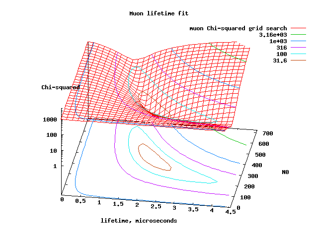
Notice that the minimum in Chi-squared is about the right value for the fit to be good at the minimum. Notice also how the values of Chi-squared get very large (many thousands ) away from the minimum.
4. Determining the Goodness of fit
The goodness of fit is determined by estimating the probability that the value of your Chisquared minimum would occur if the experiment could be repeated a very large number of times with exactly the same setup--that is, with only the sampling statistics varying on each trial. If your value of Chi-squared falls within the 68.3% (1 sigma) percentile of all the trials, then it is a good fit. In practice we can't repeat the experiment, so we need some way to estimate the value of Chi-squared that corresponds to a given percentile level (this percentile is also called the "confidence level").To determine the confidence level of a given value of Chi-squared, we first need to estimate a quantity called the number of degrees of freedom, or ND . The first guess at this is that ND = number of data values = Nd. In practice, the fact that we are constrained to fit the two parameters reduces the degrees of freedom, so
ND = (number of data values) -
(number
of parameters to fit) = Nd - Np
Once we have ND, we can now construct another
variable y which approximately transforms the Chi-squared
distribution into
a distribution with zero mean and unit standard deviation (just like a
Gaussian distribution):
(y = 3) would have only a 0.6% probability of being the correct fit.
5. Determining the standard errors on your parameters
Assuming that the shape of the Chi-squared "bowl" that you observe around your minimum Chi-squared is approximately paraboloidal in cross section close to the minimum. This is exactly true if all of your parameters are independent and if your measurement errors have a normal gaussian distribution.In this case we can think of Chi-squared as a sum of ND = Nd - Np independent gaussian distributions (the Np parameter fits constrain the distribution and reduce the amount that Chi-squared can vary). If the model we are fitting is on average always within 1 sigma of the curve, the Chi-squared value is going to equal (1* Nd ).
This is not an exact derivation, but it is a heuristic motivation as to why we use the (Chisquared+1) contour to find the standard error in the parameter, and also why the 2 and 3-sigma contours correspond to (Chisquared+4) and (Chisquared+9)--this is due to the parabolic shape around the minimum.