dy/dt = f( t , y(t) ) (1)
where the right hand side (RHS) f( t , y(t) ) is
some function of both time and the dependent variable y(t) on the left hand side
(LHS), itself a function of time. Then the 2nd order Runge-Kutta
method estimates y(t)
as follows:
y(t +
dt) = y(t) + k2
where
k2 = dt * f( t+dt/2 ,
y(t)+ k1/2 ) ,
and k1 = dt * f( t , y(t) )
and k1 = dt * f( t , y(t) )
For example, in the mass-on-a-spring
that we have considered, there are two such equations in
form (1) above:
dx/dt
= v(t)
==> f = f(t)
only, no x dependence
dv/dt = f(t) = -(k/m) * x(t) ==> also only f(t), no v(t) dependence
dv/dt = f(t) = -(k/m) * x(t) ==> also only f(t), no v(t) dependence
Why do we say they fit the form in
equation (1)? Because in each case the LHS is a
first-order differential, and the RHS is a function
that does not contain derivatives of the dependent
variable y , rather it only contains y
itself as some function of t. However,
because these are two coupled equations, we will have to
solve them together step-by-step as we did for
Euler's method, with each step for each equation
involving terms from the other equation's previous
iteration.
To apply the 2nd order RK method to our
system, we first treat the dx/dt equation:
x(t+dt)
= x(t) + k2
k2 = dt * v(t+dt/2)
= dt * (v(t) + (dv/dt)*dt/2)
= dt * (v(t) + (-k/m)x(t)*dt/2)
k2 = dt * v(t+dt/2)
= dt * (v(t) + (dv/dt)*dt/2)
= dt * (v(t) + (-k/m)x(t)*dt/2)
So it is evident that we express x(t+dt) in terms of
the original x(t)
value and an Euler's approximation term for the slope of
the x(t) curve
(which is of course v(t))
at the mid-point of the interval.
For the dv/dt equation we have:
For the dv/dt equation we have:
v(t+dt) = v(t) + k2
k2 = dt * (-k/m)* x(t+dt/2)
= dt * (-k/m)* (x(t) + (dx/dt)*dt/2)
= dt * (-k/m)* (x(t) + v(t)*dt/2)
k2 = dt * (-k/m)* x(t+dt/2)
= dt * (-k/m)* (x(t) + (dx/dt)*dt/2)
= dt * (-k/m)* (x(t) + v(t)*dt/2)
So, again, the RK2 method improves
on Euler's method by calculating the slope at the
midpoint of the interval, based on an Euler's
approximation, and then uses that to make a better
extrapolation for the endpoint of the interval,
accounting in part for the acceleration rather than
just the slope.
Lab Exercise (part 1):
Before continuing, go the pages linked here in section 4 to find a better way to program this:
4. Calling
functions from other functions: a cleaner way to
implement Runge-Kutta
5. The 4th order Runge-Kutta Method (RK4)
One can extend the approach of the 2nd order RK method to get an even more precise or robust method, using techniques similar to the Trapezoidal or Simpson's rule numerical integration, and Taylor's series approximations. RK4 may not always produce better results than RK2 (since for special cases RK2 can produce an exact solution) but it is almost always more stable, especially when there is a more complicated dependence of the equations of motion on the velocity or other parameters.
There are many good derivations of this in standard texts if you are interested. For our purposes, we will just use the RK4 method without proving it, though it will take some thought to implement it in C code.
For the same type of differential equation above, the general RK4 prescription is:
Lab Exercise (part 1):
- Using your hamonic oscillator program harmosc1a.cpp , add a new calculation to the inner loop to estimate the next value of x(t) and v(t) based on the RK2 method.
- Compare the results with the RK2 to the old version with Euler's method. Quantify the improvement by how well the energy is conserved.
Before continuing, go the pages linked here in section 4 to find a better way to program this:
4. Calling
functions from other functions: a cleaner way to
implement Runge-Kutta
5. The 4th order Runge-Kutta Method (RK4)
One can extend the approach of the 2nd order RK method to get an even more precise or robust method, using techniques similar to the Trapezoidal or Simpson's rule numerical integration, and Taylor's series approximations. RK4 may not always produce better results than RK2 (since for special cases RK2 can produce an exact solution) but it is almost always more stable, especially when there is a more complicated dependence of the equations of motion on the velocity or other parameters.
There are many good derivations of this in standard texts if you are interested. For our purposes, we will just use the RK4 method without proving it, though it will take some thought to implement it in C code.
For the same type of differential equation above, the general RK4 prescription is:
y(t+dt) = y(t)
+ 1/6 * (k1 + 2k2 + 2k3 + k4)
k1 = dt * f(t,y)
k2 = dt * f(t+dt/2, y(t)+k1/2)
k3 = dt * f(t+dt/2, y(t) + k2/2)
k4 = dt * f(t+dt, y(t)+k3)
k1 = dt * f(t,y)
k2 = dt * f(t+dt/2, y(t)+k1/2)
k3 = dt * f(t+dt/2, y(t) + k2/2)
k4 = dt * f(t+dt, y(t)+k3)
So to use RK4 in our example
above, we simply have to calculate several more
terms very much like we did for the RK2 case. In
particular, any time we are asked to calculate f(t+dt/2)
or f(t+dt)
we use an Euler's approximation, eg.: x(t+dt) =
x(t)+(dx/dt)*dt, or v(t+dt) = v(t) +
dv/dt * dt, where dv/dt is
determined by the force law.
Lab Exercise (part 2):
6. Application: The pendulum with large
amplitude oscillations
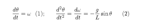
The simple pendulum has the following equation
of motion (from application of Newton's laws):

Lab Exercise (part 2):
- Using your hamonic oscillator program,
add a new calculation to the inner loop to
estimate the next value of x(t) and v(t)
based on the RK4 method, by modifying the
code for FRK2xv.cpp
to create a new function FRK4xv.cpp
- Compare the results with the RK4 to the older versions with the RK2 and Euler's methods. Quantify the change by how well the energy is conserved. Is it better or worse than RK2?
6. Application: The pendulum with large
amplitude oscillations
The simple pendulum has the following equation
of motion (from application of Newton's laws): where L is
the length, m is the mass of the bob,
g
is the local gravitational constant (g= 9.8
m/s2) and theta
is the angle through which it swings. This
equation is similar to the mass-on-a-spring
in one dimension, if we consider theta to be
analogous to x in that case. The usual way
this is solved is by assuming that theta <<
1, so sin(theta) ~ theta.
In that case the equation is formally
identical to the mass-on-a-spring.
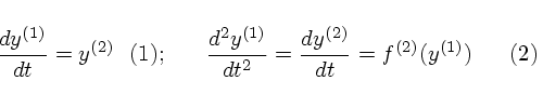
We will use the Runge-Kutta method to solve for the motion in the general case, where theta is not small--that is, where one cannot use the small-angle approximation to simplify the differential equation. In that case one must use the full form of the differential equation above, with terms cast into the General Form discussed in class and in chapter 9 of the text.
In this case, the variables can be identified with the text's standard form as follows:
In this case the functions that will need to be embedded in your parent program, and then passes as arguments to FRK2( ) are fairly simple:
Lab Assignment for Report:
7. Extra credit (15%) : Velocity
dependent drag force
Add a drag
force to either your mass-on-a-spring
harmonic oscillator or the simple pendulum
above, of the form
We will use the Runge-Kutta method to solve for the motion in the general case, where theta is not small--that is, where one cannot use the small-angle approximation to simplify the differential equation. In that case one must use the full form of the differential equation above, with terms cast into the General Form discussed in class and in chapter 9 of the text.
In this case, the variables can be identified with the text's standard form as follows:
Here
equation (1) defines the formal relation
between the angular frequency omega and
the angular variable theta, and equation
(2) is the recast form of Newton's Law
in this case. In the form given by
L&P these two equations look like
In this case the functions that will need to be embedded in your parent program, and then passes as arguments to FRK2( ) are fairly simple:
//the dx/dt function only requires returning the velocity--no action
double f_x (double t, double x, double v)
{
	return (v);
}
// Here is the actual force law
double f_v( double t, double x, double v)
{
        double retval, g, L;
	g = 0.0; // insert actual value for g
        L = 0.0; // insert actual pendulum length here
       return( retval = -g/L*sin(x));
}
Lab Assignment for Report:
- Summarize your prior exercises
where they are relevant to set the
context for the following work.
- Using your harmonic oscillator program as the template, create a new program to analyze the motion of a large-amplitude pendulum for about 10 periods or so, for a starting amplitude of 2.9 radians.
- Plot the results in a manner similar to the harmonic oscillator, including the total energy. Check energy conservation for both the Euler and RK2 methods. Compare the results to the solution for small-amplitude oscillations (eg., sinusoidal behavior).
- Plot the period of the oscillation
as a function of the starting
amplitude, from 38 degrees up to 178
degrees, in 20 degree steps (you can
just measure the period from your
graph using the cursor function of you
wish). What is the physical cause of
this behavior? (You can describe it in
qualitative terms).
7. Extra credit (15%) : Velocity
dependent drag force
Add a drag
force to either your mass-on-a-spring
harmonic oscillator or the simple pendulum
above, of the formFd = -b v
where b
is the drag coefficient (units of
kg/s). Choose a value of b
for your input parameters which damps
the oscillations down to 1/e of their
original value within about 5 periods.
Check that you conserve energy for b=0.
Check also that you can reproduce the
critically damped and overdamped cases
for some values of b.
Show some plots of the behavior.
Hint: since your equation for dv/dt now has a dependence on v, you will need to use the full Runge-Kutta terms, including the v-dependent terms shown above. You may want to separate your RK calculations into function calls to simplify the program.
Hint: since your equation for dv/dt now has a dependence on v, you will need to use the full Runge-Kutta terms, including the v-dependent terms shown above. You may want to separate your RK calculations into function calls to simplify the program.